Theory of Computation

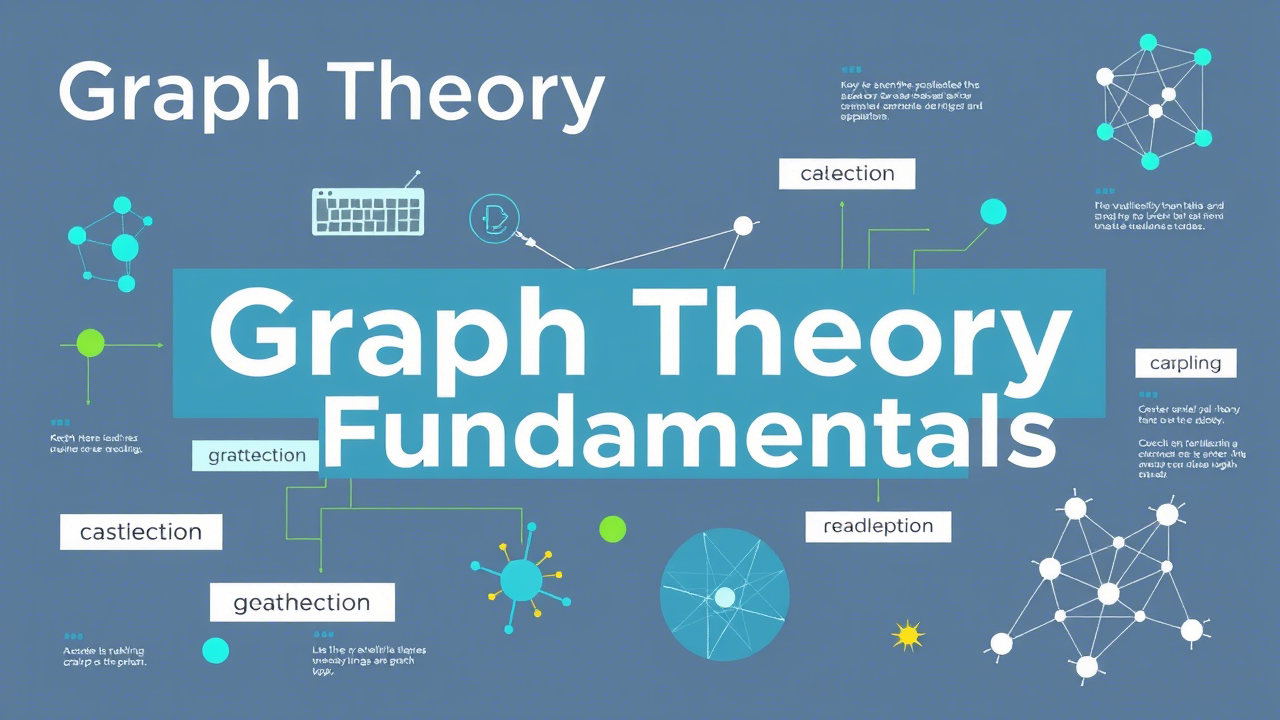
Graph Theory Fundamentals in Theory of Computation

Published

2 months ago

February 26, 2025

Graph Theory Fundamentals in Theory of Computation

Introduction

Graph theory provides a powerful framework for modeling relationships and processes in various domains, including computer science and the Theory of Computation (TOC). In this post, we will delve into the fundamental concepts of graph theory, exploring different types of graphs, their representations, and their applications in computational models and algorithms. Understanding graph theory is essential for grasping the structure of state transition diagrams in automata and the flow of computation in algorithms.

Section 1: Basic Concepts

1.1 Definition of a Graph

A graph is a mathematical structure consisting of a set of vertices (or nodes) and a set of edges that connect these vertices. Formally, a graph $G$ can be defined as $G = (V, E)$, where $V$ is the set of vertices and $E$ is the set of edges.

Example: Consider a graph $G$ with vertices $V = \{A, B, C\}$ and edges $E = \{(A, B), (B, C), (C, A)\}$. This forms a triangle where each vertex is connected to the other two.

1.2 Types of Graphs

1.2.1 Directed vs. Undirected Graphs

Undirected Graph: A graph where the edges have no direction. The edge $(A, B)$ is the same as $(B, A)$.
- Example: A social network where friendship is mutual.
Directed Graph (Digraph): A graph where the edges have a direction. The edge $(A, B)$ is not the same as $(B, A)$.
- Example: A food web where arrows indicate predator-prey relationships.

1.2.2 Weighted Graphs

Weighted Graph: A graph where each edge has an associated weight or cost.
- Example: A road network where weights represent distances or travel times.

1.2.3 Connected vs. Disconnected Graphs

Connected Graph: A graph where there is a path between every pair of vertices.
- Example: A computer network where every computer can communicate with every other computer.
Disconnected Graph: A graph where there are at least two vertices with no path between them.
- Example: A group of islands where some islands are not reachable by bridges or ferries.

Section 2: Graph Representations

2.1 Adjacency Matrix

An adjacency matrix is a square matrix used to represent a finite graph. The rows and columns correspond to the vertices, and the entries indicate whether an edge exists between the vertices.

Example:
- For a graph with vertices $V = \{A, B, C\}$ and edges $E = \{(A, B), (B, C), (C, A)\}$, the adjacency matrix would be:
```
A B C
A 0 1 1
B 0 0 1
C 1 0 0
```
2.2 Adjacency List

An adjacency list is an array of lists, where each list contains the neighbors of a vertex.
- Example:
  - ```
  A: B, C
  B: C
  C: A
```
Section 3: Applications in TOC

3.1 State Transition Diagrams in Automata

In automata theory, state transition diagrams are used to represent the behavior of finite automata. These diagrams are essentially directed graphs where vertices represent states and edges represent transitions based on input symbols.
- - - Example: A finite automaton that accepts strings ending with ‘ab’ can be represented as:
    - ```
    digraph FA {
        node [shape=circle];
        A [label="A (Start)"];
        B [label="B"];
        C [label="C (Accept)"];
        A -&gt; B [label="a"];
        B -&gt; C [label="b"];
        C -&gt; C [label="a,b"];
    }
```
3.2 Algorithm Visualization

Graph theory is also used to visualize the flow of algorithms, such as graph traversal algorithms (BFS, DFS) and shortest path algorithms (Dijkstra’s algorithm).

Note to the Reader

This post, “TOC Unit 1.1.3: Graph Theory Fundamentals for Computation,” provides a comprehensive overview of the essential concepts in graph theory and their applications in the Theory of Computation. Understanding these concepts is crucial for modeling and analyzing computational processes. In the next post, we will explore the concepts of strings, alphabets, and operations in TOC.

Prev: TOC Unit 1.1.2: Logic and Proof Techniques in Computation

Next: TOC Unit 1.2.1: Strings, Alphabets, and Operations

Up Next

Prototyping Model in Software Engineering

Don't Miss

Logic and Proof Techniques in Computation

Upendra237

Upendra237 is a self-taught engineer, programmer, mathematician, and physicist with a deep passion for knowledge and learning. Drawing from a diverse skill set and expertise in multiple disciplines, he has developed and shared a wide range of structured courses on Courseverse Online. Through these courses, Upendra237 aims to empower others by providing accessible, high-quality educational content that spans across engineering, programming, mathematics, and physics. His contributions are designed to help learners of all levels gain valuable skills and insights in these fascinating fields.

Click to comment

Theory of Computation

Logic and Proof Techniques in Computation

Published

2 months ago

February 26, 2025

Upendra237

Logic and Proof Techniques in Computation

Introduction

Logic and proof techniques are the cornerstones of rigorous reasoning in the Theory of Computation (TOC). They enable us to formally verify the correctness of algorithms, analyze the limitations of computational models, and establish the foundations of formal languages and automata theory. This post delves into the fundamental concepts of propositional and predicate logic, and explores various proof techniques that are indispensable for understanding and working with computational theories.

Section 1: Propositional Logic

1.1 Basic Concepts

Propositional logic deals with statements that can be assigned a truth value of either true or false. It provides the basic building blocks for more complex logical systems and is essential for understanding the flow of control in computational processes.

Propositions: A proposition is a declarative statement that is either true or false.
- Example: “It is raining.” (True or False)
Logical Connectives: These are operators used to combine propositions.
- Conjunction ( $\land$ ): “AND” operator.
  - Example: $P \land Q$ (True if both $P$ and $Q$ are true)
- Disjunction ( $\lor$ ): “OR” operator.
  - Example: $P \lor Q$ (True if either $P$ or $Q$ is true)
- Negation ( $\neg$ ): “NOT” operator.
  - Example: $\neg P$ (True if $P$ is false)
- Implication ( $⟹$ ): “IF…THEN…” operator.
  - Example: $P ⟹ Q$ (False only if $P$ is true and $Q$ is false)
- Biconditional ( $⟺$ ): “IF AND ONLY IF” operator.
  - Example: $P ⟺ Q$ (True if $P$ and $Q$ have the same truth value)

1.2 Truth Tables

Truth tables are used to systematically determine the truth values of compound propositions for all possible combinations of truth values of their constituent propositions.

Example Truth Table for $P \land Q$ :

$P$ $Q$ $P \land Q$

T T T

T F F

F T F

F F F

$P$	$Q$	$P \land Q$
T	T	T
T	F	F
F	T	F
F	F	F

Section 2: Predicate Logic

2.1 Basic Concepts

Predicate logic extends propositional logic by introducing quantifiers and predicates, allowing us to express more complex statements about objects and their properties.

Predicates: A predicate is a statement that contains variables and becomes a proposition when specific values are substituted for the variables.
- Example: $P (x)$ : “x is a prime number.”
Quantifiers:
- Universal Quantifier ( $\forall$ ): “For all” or “For every.”
  - Example: $\forall x \in N, P (x)$ (All natural numbers are prime – False)
- Existential Quantifier ( $\exists$ ): “There exists.”
  - Example: $\exists x \in N, P (x)$ (There exists a natural number that is prime – True)

2.2 Scope and Binding

The scope of a quantifier is the part of the formula where the quantifier applies. Variables within the scope of a quantifier are bound to that quantifier.

Example:
- $\forall x (P (x) ⟹ Q (x) )$
- Here, $x$ is bound to the universal quantifier within the scope of the implication.

Section 3: Proof Techniques

3.1 Direct Proof

A direct proof is a straightforward demonstration that a statement is true by using logical deductions from known facts or axioms.

Example: Prove that the sum of two even integers is even.
- Let $a$ and $b$ be even integers.
- Then $a = 2 m$ and $b = 2 n$ for some integers $m$ and $n$ .
- $a + b = 2 m + 2 n = 2 (m + n)$ , which is even.

3.2 Indirect Proof (Proof by Contradiction)

An indirect proof, or proof by contradiction, shows that a statement is true by assuming the opposite and deriving a contradiction.

Example: Prove that $\sqrt{2}$ is irrational.
- Assume $\sqrt{2}$ is rational, so $\sqrt{2} = \frac{p}{q}$ where $p$ and $q$ are coprime integers.
- Squaring both sides: $2 = \frac{p^2}{q^2}$ $\Rightarrow$ $2q^2 = p^2$.
- This implies $p^2$ is even, so $p$ is even. Let $p = 2k$.
- Substituting back: $2q^2 = (2k)^2 = 4k^2$ $\Rightarrow$ $q^2 = 2k^2$.
- This implies $p^2$ is even, so $p$ is even. Let $p = 2k$.
- But this contradicts the assumption that $p$ and $q$ are coprime.
- Therefore, $\sqrt{2}$ is irrational.

3.3 Mathematical Induction

Mathematical induction is a method used to prove statements about all natural numbers.

Base Case: Show the statement is true for the initial value (usually $n = 1$ ).
Inductive Step: Assume the statement is true for $n = k$ (inductive hypothesis), and prove it for $n = k + 1$ .
Example: Prove that the sum of the first $n$ natural numbers is $\frac{n(n+1)}{2}$.
- Base Case: For $n = 1$ , the sum is $1 = $\frac{1(1+1)}{2}$$ $= 1$ . True.
- Inductive Step: Assume the formula holds for $n = k$ , i.e., $1 + 2 + \dots + k = $\frac{k(k+1)}{2}$$ .
- For $n = k + 1$ :
  - $1 + 2 + \dots + k + (k + 1) = $\frac{k(k+1)}{2}$ + (k + 1)$
  - $= $\frac{k(k+1)+2(k+1)}{2}$$
  - This matches the formula for $n = k + 1$ .
- Therefore, by induction, the formula holds for all natural numbers.

Section 4: Applications in TOC

Logic and proof techniques are fundamental in various aspects of TOC:

Algorithm Correctness: Proving that an algorithm produces the correct output for all valid inputs.
Complexity Analysis: Establishing the time and space complexity of algorithms using logical reasoning.
Automata Theory: Defining the behavior of automata using logical conditions and transitions.

Note to the Reader

This post, “TOC Unit 1.1.2: Logic and Proof Techniques in Computation,” provides a comprehensive overview of the essential logic and proof techniques used in the Theory of Computation. Understanding these concepts is crucial for rigorous analysis and formal verification in computational theories. In the next post, we will explore the basics of graph theory and its applications in TOC.

Prev: TOC Unit 1.1.1: Sets, Relations, and Functions | Foundations of Computation

Next: TOC Unit 1.1.3: Graph Theory Fundamentals for Computation

Theory of Computation

Sets, Relations, and Functions | Foundations of Computation

Published

2 months ago

February 24, 2025

Upendra237

Sets, Relations, and Functions in Theory of Computation

Introduction

In the realm of Theory of Computation (TOC), mathematical rigor forms the bedrock for understanding abstract computational models. This post delves into sets, relations, and functions—fundamental concepts that underpin automata theory, formal languages, and computability. By grasping these principles, you’ll build a robust framework for analyzing algorithms, languages, and computational limits.

Section 1: Sets

1.1 Definition and Types

A set is an unordered collection of distinct objects, known as elements or members. Sets are foundational in TOC for defining languages, alphabets, and state spaces.

Notation:
- Roster Method: $A = {1, 2, 3}$ .
- Set-Builder Notation: $B = {x ∣ x is a prime number}$ .
Types of Sets:
- Finite Set: Contains a countable number of elements (e.g., $C = {a, b, c}$ ).
- Infinite Set: Contains infinitely many elements (e.g., $N = {1, 2, 3, \dots}$ ).
- Empty Set: Contains no elements ( $\emptyset$ ).
- Singleton Set: Contains exactly one element (e.g., $D = {5}$ ).

1.2 Set Operations

Set operations are critical for constructing complex languages and analyzing computational models.

Union ( $\cup$ ):
- Definition: $A \cup B = {x ∣ x \in A or x \in B}$ .
- Example: If $A = {1, 2}$ and $B = {2, 3}$ , then $A \cup B = {1, 2, 3}$ .
Intersection ( $\cap$ ):
- Definition: $A \cap B = {x ∣ x \in A and x \in B}$ .
- Example: $A \cap B = {2}$ .
Complement ( $A^{'}$ ):
- Definition: All elements not in $A$ , relative to a universal set $U$ .
- Example: If $U = {1, 2, 3, 4}$ and $A = {1, 2}$ , then $A^{'} = {3, 4}$ .
Cartesian Product ( $A \times B$ ):
- Definition: Ordered pairs $(a, b)$ where $a \in A$ and $b \in B$ .
- Example: $A = {a}$ , $B = {1, 2}$ → $A \times B = {(a, 1), (a, 2)}$ .

1.3 Set Identities

These identities simplify expressions in automata construction and language theory:

Commutativity: $A \cup B = B \cup A$ , $A \cap B = B \cap A$ .
Associativity: $(A \cup B) \cup C = A \cup (B \cup C)$ .
Distributivity: $A \cap (B \cup C) = (A \cap B) \cup (A \cap C)$ .

Section 2: Relations

2.1 Definition and Types

A relation is a subset of the Cartesian product of two sets, denoting connections between elements.

Binary Relation: A relation between two sets $A$ and $B$ , e.g., $R \subseteq A \times B$ .
Example: $R = {(a, 1), (b, 2)}$ relates letters to numbers.

2.2 Special Relations

Equivalence Relation: A relation that is reflexive, symmetric, and transitive.
- Example: Modular arithmetic ( $a \equiv b (mod n)$ ).
Partial Order: A relation that is reflexive, antisymmetric, and transitive.
- Example: Subset relation ( $\subseteq$ ) on power sets.

2.3 Representation

Matrix Representation:
- For $R \subseteq A \times B$ , use a matrix where rows = $A$ , columns = $B$ , and entries = 1/0 for relation presence.
Digraph Representation:
- Nodes represent elements; edges represent relation pairs.
- Example: Graphviz code for a relation:
- ```
digraph Relation {
a -> 1;
b -> 2;
}
```

Section 3: Functions

3.1 Definition and Types

A function (or mapping) assigns exactly one output to each input.

Injective (One-to-One): No two inputs map to the same output.
- Example: $f (x) = 2 x$ (maps integers to even numbers).
Surjective (Onto): Every output has a corresponding input.
- Example: $f : N \to N$ , $f (x) = x$ (identity function).
Bijective: Both injective and surjective.
- Example: $f (x) = x + 1$ on $Z$ .

3.2 Composition and Inverses

Function Composition:
- $(g \circ f) (x) = g (f (x))$ .
- Example: $f (x) = x + 1$ , $g (x) = 2 x$ → $g (f (x) ) = 2 (x + 1)$ .
Inverse Function:
- $f^{- 1} (y) = x$ if $f (x) = y$ .
- Example: $f (x) = x^{3}$ has inverse $f^{- 1} (y) = 3 y$ .

Section 4: Applications in TOC

Alphabets and Strings:
- An alphabet $Σ$ is a finite set (e.g., $Σ = {a, b}$ ).
- Strings are finite sequences from $Σ$ (e.g., “aab”).
State Transition Functions:
- In finite automata, $δ : Q \times Σ \to Q$ defines state transitions.
Language Recognition:
- Functions map strings to accept/reject decisions.

Summary

This post laid the groundwork for TOC by exploring sets, relations, and functions. These concepts are indispensable for modeling computation, defining languages, and analyzing algorithms. In the next post, we’ll delve into logic and proof techniques, essential for rigorous analysis in TOC.

Next: [TOC Unit 1.1.2: Logic and Proof Techniques in Computation]

Note to the Reader

This post is part of the TOC Unit 1: Foundations of Computation series. Unit 1.1.1: Sets, Relations, and Functions. It covers the essential concepts of sets, relations, and functions, which are crucial for understanding more advanced topics in automata theory and formal languages. If you have any questions or need further clarification, feel free to leave a comment below.

Fashion8 years ago

These ’90s fashion trends are making a comeback in 2017

Fashion8 years ago

According to Dior Couture, this taboo fashion accessory is back

Entertainment8 years ago

The old and New Edition cast comes together to perform

Business8 years ago

Uber and Lyft are finally available in all of New York State

Entertainment8 years ago

The final 6 ‘Game of Thrones’ episodes might feel like a full season

Entertainment8 years ago

‘Better Call Saul’ has been renewed for a fourth season

Politics8 years ago

Congress rolls out ‘Better Deal,’ new economic agenda

Entertainment8 years ago

Meet Superman’s grandfather in new trailer for Krypton

Course Verse

Graph Theory Fundamentals in Theory of Computation

Introduction

Section 1: Basic Concepts

1.1 Definition of a Graph

1.2 Types of Graphs

1.2.1 Directed vs. Undirected Graphs

1.2.2 Weighted Graphs

1.2.3 Connected vs. Disconnected Graphs

Section 2: Graph Representations

2.1 Adjacency Matrix

2.2 Adjacency List

Section 3: Applications in TOC

3.1 State Transition Diagrams in Automata

3.2 Algorithm Visualization

Note to the Reader

You may like

Leave a Reply Cancel reply

Leave a Reply

Theory of Computation

Logic and Proof Techniques in Computation

Introduction

Section 1: Propositional Logic

1.1 Basic Concepts

1.2 Truth Tables

Section 2: Predicate Logic

2.1 Basic Concepts

2.2 Scope and Binding

Section 3: Proof Techniques

3.1 Direct Proof

3.2 Indirect Proof (Proof by Contradiction)

3.3 Mathematical Induction

Section 4: Applications in TOC

Note to the Reader

Theory of Computation

Sets, Relations, and Functions | Foundations of Computation

Introduction

Section 1: Sets

1.1 Definition and Types

1.2 Set Operations

Section 2: Relations

2.1 Definition and Types

2.2 Special Relations

2.3 Representation

Section 3: Functions

3.1 Definition and Types

3.2 Composition and Inverses

Section 4: Applications in TOC

Summary

Note to the Reader

Artificial Intelligence Syllabus

Internet of Things (IoT) Syllabus

Requirement Definition and Specification in Software Engineering

These ’90s fashion trends are making a comeback in 2017

According to Dior Couture, this taboo fashion accessory is back

The old and New Edition cast comes together to perform

Illinois’ financial crisis could bring the state to a halt

The final 6 ‘Game of Thrones’ episodes might feel like a full season

New Season 8 Walking Dead trailer flashes forward in time

Trending

Leave a Reply
Cancel reply